Solved Paper-Design and Analysis of Algorithm

1. Choose the correct option:                                  (10×1=10)

(i) Big Oh notation gives

(a) Upper Bound

(b) Lower Bound

(c) Strictly Upper bound

(d) Strictly Lower Bound

(ii) Which of the following method is used to solved a recurrence?

(a) Substitution Method

(b) Master Method

(c) Changing Variable

(d) All of the above

(iii) Which sorting adopt divide and conquer technique?

(a) Merge Sort

(b) Selection Sort

(c) Bubble Sort

(d) Insertion Sort

(iv) Which Data Structure is used to perform Recursion?

(a) Queue

(b) Stack

(c) Priority Queue

(d) All of the above

(v) Time complexity of matrix chain multiplication problem is

(a) O(n)

(b) O(n²)

(c) O(n³)

(d) None of these

(vi) The running time of an algorithm is given by

(a) Total number of basic operations performed by the algorithm

(b) Total number of statements

(c) Maximum time taken to execute

(d) None of the above

(vii) If f(n)=θ(g(n) then

(a) 0≤c₁g(n)≤f(n)≤c₂g(n) for all n≥n₀

(b) 0≤f(n)≤c₂g(n) for all n≥n₀

(c) 0≤c₁g(n)≤f(n) for all n≥n₀

(d) None of the above

(viii) In greedy method which type of solution is generated

(a) Optimal solution

(b) Worst solution

(c) Best solution

(d) All solutions

(ix) In a knapsack problem, if a set of items are given each with a weight and a value, the goal is to find the number of items that __________ the total weight and the total value.

(a) Maximizes, Maximizes

(b) Minimizes, Minimizes

(c) Maximizes, Minimizes

(d) Minimizes, Maximizes

(x) Which of the following sorting algorithms is the fastest?

(a) Merge sort

(b) Quick sort

(c) Insertion sort

(d) Bubble sort

2. (a) Define Algorithm. Discuss key characteristics of algorithm.  (5)

Ans: An algorithm is a well-defined set of steps used to perform a specific task. It is a finite sequence of instructions to solve a problem or carrying out a computation. Algorithm describes how to solve a problem.

It is a step-by-step procedure or set of rules designed to perform a specific task or solve a particular problem. Algorithm refers to the set of finite instructions to be followed in calculations or other problem-solving operations.

Key Characteristics of Algorithm:

An algorithm should have the following characteristics:

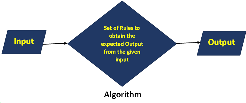
Input: An algorithm requires some input values. Algorithms take input which is the data or information they operate on. The input can vary from problem to problem and is essential for the algorithm’s operation.

Output: There should be at least one output produced. Algorithm produces output which is the solutions or result to the problem. The output should be in a format that is understandable and useful to the user.

Definiteness:  Each step of an algorithm should be well-defined, clear and simple. Algorithm should be clear and unambiguous. There should be no ambiguity in how to execute each step.

Finiteness: Here, finiteness means that the algorithm should contain a limited number of instructions. The number of steps in an algorithm is finite. Algorithms should terminate after a finite number of steps. They should not run indefinitely. This ensures that the algorithm’s execution will eventually complete.

Effectiveness:  An algorithm must be effective in that it can solve the problem or complete the task for any valid input. Every instruction must be basic i.e., simple instructions.

Feasible: Algorithm must be capable of execution within a reasonable amount of time and resources. The algorithm must be simple, generic and practical such that it can be executed with the available resources. They shouldn’t be overly complex and inefficient.

(b) State the different methods of analyzing algorithm. Which one is prefer most? Justify.       (3)                                            

Ans: Analysis of algorithm is the process of analyzing the problem-solving capability of the algorithm in terms of the time and size required (the size of memory for storage while implementation).

There are several methods for analyzing algorithms, each providing different insights into their performance. The choice of method depends on the goals of the analysis and the characteristics of the algorithm. Here are some common methods for analyzing algorithms:

Asymptotic Analysis: Focuses on the growth rate of the algorithm as the input size approaches infinity.

• Time Complexity: Describes the growth rate of an algorithm’s running time as the input size increases.
• Space Complexity: Analyzes the growth rate of the space required by an algorithm.

Empirical Analysis: Involves running the algorithm on real-world inputs and measuring actual performance, providing practical insights but often less precise than theoretical analysis.

Average, Best, and Worst-Case Analysis: Examines thealgorithm’s performance under different scenarios- best case, worst case and average case- considering various input distributions.

• Best Case Analysis: Examines the lower bound on the performance, which is achieved for the best possible input.
• Worst Case Analysis: Focuses on the upper bound of the performance, considering the input that leads to the maximum running time or resource usage.
• Average Case Analysis: Considers the average performance over all possible inputs.

Amortized Analysis: Evaluates the average time taken per operation over a sequence of operations, providing a more accurate estimate of the overall performance.

Preference and Justification:

The preference for a particular method depends on the specific context Asymptotic analysis is often preferred because it provides a high-level view of an algorithm’s efficiency and is independent of hardware and implementation details. Big-O notation, a common notation in asymptotic analysis, allows for a quick comparison of algorithms and is widely used in theoretical computer science.

Empirical analysis is valuable for understanding the practical performance of an algorithm in real-world scenarios. It takes into account factors that may be difficult to capture in theoretical analyses, such as constant factors, hardware differences, and peculiarities of specific inputs.

In practice, a combination of both asymptotic analysis and empirical analysis is often used. Theoretical analysis helps in understanding the algorithm’s behavior in the abstract, while empirical analysis provides insights into its performance in real-world scenarios. The preference for one over the other depends on the specific goals of the analysis and the available resources.

(b) Define B tree. Mention the basic operations that can be performed on B tree.              (2+5=7)

Ans: A B-tree is a balanced search tree in which each node can have multiple keys and child pointers. The keys in a node are stored in sorted order, and the number of keys in a node is within a certain range. This range is determined by a parameter called the order of the tree, denoted by t. A B-tree of order t satisfies the following properties:

1. Each internal node has at most 2t−1 keys and at least t−1 keys.
2. Each internal node has at most 2t child pointers.
3. All leaves are at the same level.
4. Every non-leaf node contains k−1 keys and k child pointers.

Basic Operations:

Search:

Start at the root and recursively search the B-tree like a binary search tree until finding the desired key or determining that it is not present.

Insertion:

• Start with a search to find the correct position for the new key.If the node is not full, insert the key.

• If the node is full, split it and promote the middle key to the parent, recursively handling overflow issues.

• Deletion:
  • Start with a search to find the key to be deleted.
  • If the key is in a leaf, delete it directly.
  • If the key is in an internal node, find its predecessor or successor from its child, replace the key with the predecessor/successor, and recursively delete the predecessor/successor.
• Traversal:
  • In-order traversal of a B-tree produces a sorted sequence of keys.

• Range Queries:
  • B-trees efficiently support range queries, where a range of keys needs to be retrieved.

• Splitting and Merging:
  • When a node becomes full during an insertion, it is split into two nodes, and a key is promoted to the parent.
  • When a node becomes less than half full during a deletion, it may be merged with a sibling node.

B-trees provide efficient disk-based storage and retrieval due to their ability to minimize disk I/O operations and maintain balance during insertions and deletions.

6. (b) What is coin changing problem? Explain how greedy algorithm can be used to solve this problem.        (5)

Ans: The coin changing problem is a classic optimization problem in which the goal is to make change for a given amount using the fewest possible coins. Given a set of coin denominations and a target amount, the objective is to find the minimum number of coins needed to make up that amount. This problem is often encountered in real-world scenarios, such as making change in vending machines or cash transactions.

Here’s a formal definition of the problem:

Input:

• A set of coin denominations {d₁​, d₂​,….,d_k​}, where d_i​ is the denomination of the i-th coin.
• A target amount A.

Output:

• The minimum number of coins needed to make change for A.

Greedy Algorithm for Coin Changing:

The greedy algorithm for the coin changing problem is based on the idea of always selecting the largest denomination coin that is less than or equal to the remaining amount. Here are the steps:

1. Sort the coin denominations in decreasing order.
2. Initialize a variable to store the total number of coins used (let’s call it numCoins).
3. Iterate through the sorted denominations:
   • At each step, if the current denomination is less than or equal to the remaining amount, add it to the solution and subtract it from the remaining amount.
   • Repeat this process until the remaining amount becomes zero.

The greedy algorithm works well for certain coin systems, such as the U.S. coin system (where the denominations are 1, 5, 10, 25 cents). However, it may not always provide the optimal solution for arbitrary coin systems.

7. (a) Define P, NP and NP Complete problems.                                2×3=6

Ans: In computational complexity theory, P, NP, and NP-complete are classes of decision problems, where a decision problem is a problem with a yes/no answer. These classes help classify problems based on their inherent difficulty and the efficiency of algorithms that solve them.

P (Polynomial Time): P is the class of decision problems for which there exists an algorithm that can find a solution in polynomial time with respect to the size of the input. P represents problems that can be solved efficiently in polynomial time. The class P consists of decision problems for which a solution can be verified by a deterministic Turing machine in polynomial time. These problems are considered efficiently solvable. Problems in P are considered “easy” or “tractable” in terms of computation, because their solutions cab be found efficiently.

Example: Sorting a list of numbers, finding the shortest path in a graph, etc. Finding the maximum element in an array is a problem in P because an algorithm can do this in linear time(O(n)).

NP (Non-deterministic Polynomial Time): NP is the class of decision problems for which a given solution can be verified quickly in polynomial time. Or other words, if we have a candidate solution, we can efficiently check its correctness in polynomial time. However, finding the solution itself may not be easy. NP problems are decision problems for which a proposed solutions can be checked quickly but finding the solution itself may not be as straightforward. NP represents problems for which solutions can be verified quickly, though finding solutions is not necessarily efficient.

Example: The travelling salesman problem is in NP because given a solution, one can quickly verify if it is correct.  The traveling salesman problem, where checking if a given route is the shortest can be done in polynomial time, but finding the shortest route is a harder problem.

NP-Complete (Non-deterministic Polynomial Time Complete): A decision problem is NP-complete if it is NP and has the property that any problem in NP can be reduced to it in polynomial-time. An NP-complete problem is one that is as “hard” as the hardest problems in NP. NP-Complete represents the most difficult problems in NP, and if a polynomial time solution is found for any NP-complete problem, it implies polynomial-time solutions for all problems in NP.

A problem is NP-complete if it satisfies two conditions:

1. It belongs to the class NP: This means that given a proposed solution, we can verify whether it is correct or not in polynomial time.
2. It is as hard as the hardest problems in NP: More precisely, if we could find a polynomial-time algorithm to solve any NP-complete problem, we could use that algorithm to solve any problem in NP in polynomial time. This is often referred to as polynomial-time reducibility or polynomial-time transformation.

Example: The Boolean satisfiability problem (SAT) is a classic NP-complete problem. If we could efficiently solve SAT, we could efficiently solve any problem in NP.

NP-complete problems are some of the most challenging problems in computational complexity theory and if an efficient algorithm exists for any NP-Complete problems, it could imply that efficient algorithm exists for all problem in NP.

(b) Analyze the running time of merge sort using recurrence tree method.                (9)

Ans: The recurrence tree method is a technique for analyzing the time complexity of recursive algorithms by representing the recursive calls as nodes in a tree. Let’s analyze the running time of the merge sort algorithm using the recurrence tree method.

Merge Sort is a divide-and-conquer algorithm that works as follows:

1. Divide: Divide an array of n elements into two arrays of n/2 elements each.
2. Conquer: Sort the two arrays recursively
3. Combine: Merge the two sorted arrays into a single sorted array.

The recurrence relation for the time complexity of Merge Sort algorithm can be expressed as follows:

T(n)=2T(n/2) + O(n)

Here, T(n) represents the time complexity of Merge Sort for a list of size n, and O(n) represents the time taken for the merging step.

This recurrence relation represents the time complexity of merge sort. Here’s how the recurrence tree method helps in analyzing the running time:

1. Level 0: The original problem of size n.
2. Level 1: Two subproblems, each of size n/2, created in the “Divide” step.
3. Level 2: Four subproblems, each of size n/4.
4. …

This process continues until we reach subproblems of size 1.

At each level, the total work done is O(n) due to the merging step. The total number of levels is log₂​n because we are dividing the problem size by 2 at each level. So, the total work done is the sum of the work at each level:

T(n)=log2​n⋅O(n)

Therefore, the overall time complexity of merge sort is O(nlogn) when analyzed using the recurrence tree method. This makes merge sort a very efficient algorithm for sorting.